We now have enough data to make a plot showing how the period of KIC 9832227 has (or has not) been changing since we started observing at the end of November. And that plot looks like this:

In this graph, the horizontal x-axis is time (the date), and the vertical axis is the orbital period of the binary. Two scales are shown for the vertical axis. On the left is period in hours, and on the right is the period in seconds relative to 11 hours exactly. (So, on the right, a period of 11h00m05s will plot as +5 and a period of 10h59m55s will plot as -5.)

Each measurement of the period has a red dot and a vertical bar that shows the uncertainty of the measurement. A short vertical bar means that this particular measurement is more certain (less fuzzy) than a point with a long vertical bar. (There’s one vertical bar without a red dot. That’s because the red dot falls below the bottom of the plot.)

Measurements come from pairs of observing sessions. Whenever two observing sessions include data from the same part of the binary’s orbit, we can estimate the average period of the binary in between those two observing sessions by finding the value of the period that gives the best (smoothest) overlap when that overlap data is plotted in the phase plot. The time of that measurement is taken to be the time halfway between the two observing sessions.

Measurement uncertainty is driven by several things. First, if the data is noisy (lots of data scatter in the brightness measurements), then the timing uncertainty tends to be bigger. Second, if the number of days between the two observing sessions is big, then the uncertainty tends to be smaller, since the timing uncertainty is divided by the number of orbits that have been completed. If the overlapped data covers multiple hours, the uncertainty will be smaller than if the overlap only lasts a few minutes. Finally, if the brightness doesn’t change very quickly during the overlap period, then the uncertainty can be high. (There’s one overlap period where the brightness is essentially constant. I had to throw out this measurement.)

And the green line is the weighted straight line best fit to the data (a so-called weighted linear regression). (“Weighted” means that measurement uncertainty (the vertical uncertainty bars) have been taken into account in finding the best fit — points with small uncertainty have a bigger influence on the green line than points with large uncertainty.) If that line has a positive slope, then the period is getting longer (and the stars are spiraling outward from each other); a negative slope means that the two stars are spiraling inward. The current green line has a slope of +0.007 seconds/orbit, but has an uncertainty several times bigger than that. Our data so far rules out nothing, and is consistent with the orbit being stable, with them spiraling inward, and with them spiraling outward.

So, we just don’t know yet! We need more data, more images of KIC 9832227. (We currently have 1,934 brightness measurements, one per image.)

Waiting for some more bad weather to clear, so let’s talk about time …

There are a handful of different time zones that are relevant to this project:

Local Time: Right now, local time for me is Eastern Standard Time. This is the time zone that I use for planning telescope observations. I can easily look up the time of sunset and time of sunrise in the newspaper; both are most easily found as EST. The clock in my bedroom that tells me when to wake up, go outside, and shut down the telescope is set to local time.

Coordinated Universal Time (UTC): UTC is the “master” time that controls my computers. Each computer (including the telescope mount) is synchronized to UTC time to within a millisecond or so. (Right now, EST is 5 hours earlier than UTC.) Each image includes the UTC time that the camera shutter opened. (Although the time that I actually use when I make my plots is the time of the midpoint of the exposure: halfway between the time that the shutter opened and the time that the shutter closed.)

Julian Days: Astronomers are fundamentally lazy, and will invent things in order to avoid work. One of the unpleasant tasks that astronomers like to avoid is answering a question such as the following:

How long is it between 7am (UTC) on January 14, 2018 and 9pm (UTC) on March 11, 2018?

Yuk. And an additional yuk because you have to figure out whether there’s a February 29 leap day in there somewhere.

And so astronomers invented “Julian Days”. The Julian Day calendar started on January 1, 4713BC, and has been counting the days ever since, one day at a time. I am drafting this post on Julian Day 2,458,861. Using Julian Days makes counting intervals really easy.

Further, astronomers will frequently use decimal parts of the Julian Day to measure time within the day. So, for example, astronomers use a fractional part of .000 to refer to noon. So, today at noon is Julian Day 2,458,861.000. And, today at midnight will be Julian Day 2,458,861.500. The time of the first image that I grabbed of KIC 9832227 is 2,458,814.51415.

However, when I go to calculate the orbit time of KIC 9832227, I don’t use UTC or Julian Day directly, because it doesn’t take into account the speed of light. As far back as Galileo, astronomers noticed that the motion of things in the sky (Galileo noticed it with the motion of the moons of Jupiter) sometimes seems to happen up to 8 minutes earlier than expected and sometimes seems to happen up to 8 minutes later than expected. This led to an early understanding that the radius of the Earth’s orbit around the sun is about 8 “light-minutes”. When the Earth is close to the object being observed, light travels some 93 million miles less than when the Earth is at the halfway point in its orbit, and it takes about 8 minutes for light to travel that distance.

And so astronomers “invented” something called “heliocentric time.” This is the time that an observer working at the center of the sun (and using a clock synchronized to UTC) would observe an event. It’s simply UTC with up to 8 minutes added or subtracted depending on which direction you’re looking. You would think that this would compensate for the 8 minute speed-of-light problem, but it doesn’t quite work…

Instead, I’m using a time called Barycentric Dynamical Time (BJD_TDB). This is very close to heliocentric time, but it acknowledges that the Earth doesn’t orbit around the center of the sun. Instead, the Earth orbits around the solar system’s barycenter: the effective center of mass of the entire solar system. The barycenter is offset from the center of the sun, mostly due to Jupiter and Saturn. (The Wikipedia article on barycenter is pretty cool, with animations.) And so Barycentric Dynamical Time takes the speed of light into account based on what an observer located at the solar system’s barycenter would see. This is the time that I actually use when calculating the KIC 9832227 orbital characteristics.

And that brings us to the final “timezone” …

Orbit Time: This is an odd clock; it measures time in the KIC 9832227 orbit. Orbit Time goes from 0 to 10 hours 59 minutes 26.7 seconds (which is how long it takes the two stars in KIC 9832227 to return to the exact same spot that they had at Orbit Time zero), and then resets back to zero. Traditionally, astronomers set the zero of the Orbit Time clock at the midpoint of the deepest minimum in the binary star’s lightcurve. Since I didn’t know when that was when we started observing KIC 9832227, I arbitrarily set Orbit Time to zero at the midpoint of the very first exposure that I made of KIC 9832227 (as measured in Barycentric Dynamical Time). At some point in the future, maybe, I’ll reset my definition of Orbit Time to coincide with that minimum, but I don’t yet have a reason to do so. (And because I’m basically lazy, I’m going to do nothing until I’m forced to make a change.) This Orbit Time is the time that I’ve been using in the Phase Diagram plots that I’ve shown in prior posts.

Yuk. We’re getting into our full-blown winter weather pattern, which makes observing more difficult. Nonetheless, sessions 6 (December 24) and 7 (January 1) are noteworthy because they contain the first “dual” session observing KIC 9832227. On both days, I had the telescope observe KIC 9832227 from sunset (about 5pm) until “star-set” (about 9pm) and then do another observing run from “star-rise” (about 4am) until sunrise (about 6:30am). (And from 9pm to 4am I did my other astronomy observing projects.) Bad morning weather prevented anything useful from the morning session on Christmas Morning, but on January 1 there is some good data from both the evening run and the morning run.

There are now over 1,700 data points in the combined light curve:

My original reason to study KIC 9832227 wasn’t to create a lightcurve, but to measure the timing of this star to see if I could detect changes in the period over time: are the stars spiraling toward each other?

Observing session 5 was a good session, although I started well after sunset because of another commitment that flowed into making dinner and other chores. So, session 5 was a little bit short. But all those earlier problems with horizon and blurry images have now been solved, so although I only had 2 or 3 hours of observing time with this session, the image quality is somewhat above average.

The new points (a dark red in this graph, from about 4 hours to about 7 hours in the orbital cycle ) overlap points from other sessions, which means that we should be able to extract a timing measurement.

My timing spreadsheet gives me an orbital cycle time of 0.45790008182729164 days. That is 10 hours, 59 minutes, 22.57 seconds. The American Association of Variable Star Observers lists its orbital cycle time as 0.4579485 days. My measured timing is 4.18 seconds faster than the AAVSO’s time. However, I don’t (yet) have much confidence in my timing. The associated timing spreadsheet graph is quite broad and the points show lots of scatter. More data and editing/removing some of the relatively wild data points might tighten things up.

We’ll see.

Meanwhile, I think it’s really cool to be able to measure the orbital cycle time down to the second, despite using 30-second-long exposures. Just goes to show that if you have enough data points and are careful with your clock (the computer clock used to attach time to each exposure is kept synchronized with Coordinated Universal Time (UTC) to a few milliseconds), you can make surprisingly precise statements about orbits. Oh, and I am adjusting for the speed of light, which is an important correction in this measurement. (But one that I’ll cover in some future blog post.)

Sunday December 15: Observing Session 4

Once again, weather interfered. Had to throw away at least an hour’s worth of images due to clouds. Nevertheless, we’ve now accumulated a grand total of 1,040 usable images, each of which provides one brightness measurement. Let’s see what we can do with that.

This (unimpressive) graph shows the raw data. (Remember that star brightness measured in magnitudes seems to be backwards: bigger magnitude numbers are fainter than smaller magnitude numbers.) Each of the 1,040 data points is plotted in green as a brightness (y axis) against the time the image was exposed (x axis). The numbers on the x axis are “Julian Dates,” the standard way that astronomers manage observation times. A day’s Julian Date is simply the number of days that have elapsed since the Julian Calendar reference date: Monday, January 1, 4713 BC. There’s nothing useful to be gleaned from this graph.

But, there’s another way to graph this data, one that takes advantage of KIC9832227’s orbital period of about 11 hours. Instead of plotting each point in “absolute time,” we can plot each point in “orbital time,” which goes from 0 to 11 hours. That results in the following graph:

Each observing run is plotted in a different color. These four runs give us almost complete coverage of an entire orbit. (Although there’s still a lot of data scatter as a result of all the poor weather we’ve encountered.) Observations and things to ponder:

• The two minima don’t match brightness. The minimum at 3 hours has a brightness of about 12.48 and the minimum at 8.2 hours has a brightness of about 12.51. (That makes the minimum at 3 hours the secondary eclipse and the minimum at 8.2 hours the primary eclipse.) Because the two minima don’t match, the two stars must have different brightness/size.
• The maximum that’s around 5.7 hours isn’t in the “middle” of the two minima. It takes longer to get from the 3-hour secondary eclipse to the maximum than it takes to get from the maximum to the 8.2 hour primary eclipse. This means that the two stars are in an elliptical orbit; if the orbit was circular, the timing would match. [Update: the more I stare a this, the more I’m uncertain about where the “middle” is. Maybe need more data before this becomes clear??]
• There are several parts of the orbit where measurements from two observing sessions overlap. This provides an opportunity for our own measurement of orbital period, which I’ll address in a subsequent post.
• There’s no part of the lightcurve where brightness “stands still.” This is further confirmation that these two stars are a contact binary, actually touching each other.

All in all, this is pretty cool. Despite all the bad weather and problems with fuzzy, blurred, near-the-horizon, out-of-focus images, we’ve succeeded in creating a graph showing how brightness changes over time for this close binary star. That’s neat.

5pm Thursday, December 12

I’m ready to test things. I’ve made a series of software changes:

• When the software is unable to measure the blurriness of an image (because it’s too blurry), the rest of the software will correctly ignore the focus of that image.
• All blurriness measurements are adjusted based on the image’s height above the horizon — this should prevent the software from getting upset because images are getting fuzzy solely because they are close to the horizon.

Weather forecast is lousy, but there may be a few hours of thin, scattered clouds right after sunset. I can use that to try and test this new software. Let’s see what happens……

Aha! (4 hours later)

Yes, the clouds rolled in. However, things look much better than before. I have a total of 207 images, although only the first 100 are cloud-free. However, all except the last 6 images will yield a brightness measurement. Focus remained good throughout. The resulting light curve looks like this (the arrival of the clouds is really obvious):

Pretty soon we’ll have enough data points to do something interesting . . .

5pm on Wednesday, December 11

By the way, I’ve added a spot on the blog’s cover page where I’ve listed all the blog entries in order, since it can be hard to figure out how to read these entries from beginning to end and they probably don’t make a lot of sense out of order.

Weather looks good, so let’s try again. What I’ve figured out (and what will guide this observing run):

• As stars move toward the horizon, I can get reasonably acceptable images until the airmass reaches about 5.
• An airmass of 5 corresponds to an altitude above the horizon of 11 degrees. (Make a fist, hold your fist at arm’s length so that the bottom of your fist aligns with the horizon. The top of your fist will now be about 10 degrees above the horizon.)

So, knowing that the magic location in the sky is about 11 degrees above the horizon, I’m going to stop talking about airmass, and just talk about altitude above the horizon. I’ll use a spreadsheet to create a graph of KIC9832227’s altitude above the horizon tonight:

KIC9832227 will be above my magic 11-degree altitude from sunset until about 10pm, and then will rise back up above 11 degrees around 5:30am. Morning twilight will swamp images by 6:30am, so there are about 5 useful hours after sunset and 1 useful hour before sunrise. I will set up to run continuously until 10pm, and won’t bother with an early morning run (for now).

Curious minds are looking for answers: What was the airmass problem? And just what is airmass, anyway? Why did the quality of the images get worse and worse as the night went on? Is there anything different we can (or should) do next time?

Airmass: What is it?

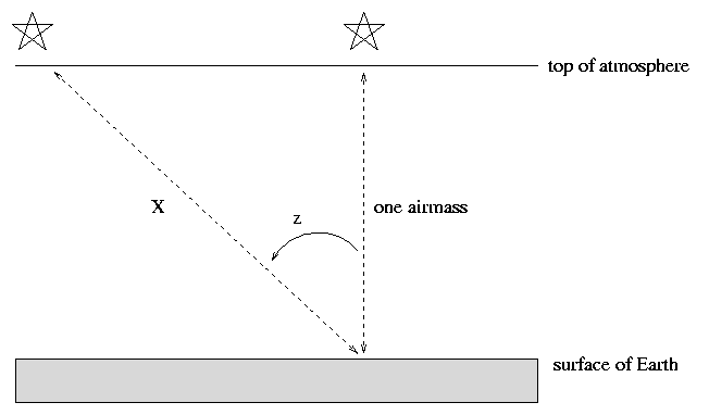
When you look at a star that is exactly right above you, right at the zenith (the highest point in the sky above your head), you are looking through exactly one thickness of the earth’s atmosphere.

But when you look at a star somewhere else in the sky, not directly overhead, but closer to the horizon, you are looking through extra atmosphere. Take a look at this diagram (from a course offered at Rochester Institute of Technology):

There’s more air along the line X than there is along the line labeled “one airmass.” Whenever I store an image that I’ve taken at my telescope, I also store an “airmass” number with the image. The airmass number can be as small as 1.0 when the telescope is pointed directly overhead. As the telescope gets closer to the horizon, the airmass number gets bigger. To calculate airmass, I first calculate how high above the horizon the telescope is pointed, then use a complex formula to estimate the airmass.

So, under what conditions can the complex formula generate a floating point computation error? Only one way: if the height above the horizon is negative; in other words, if the telescope is pointed toward the ground.

Hmmm. Why would we do this? Where in the sky is KIC 9832227 located? Well, we get one hint by looking at the value of airmass that was attached to each of the images from that night. Plotting those points creates the following graph:

Aha! I usually set a limit of something between an airmass of 5.0 (usually) and an airmass of 10.0 (rarely) as the limit of what I will accept. Once airmass gets above about 5, the telescope is pointed too close to the horizon for good pictures. An airmass of 30+ is ridiculous.

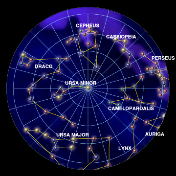
All the stars in our sky appear to rotate around the North Star (Polaris) once per day. The stars that are closest to the North Star never seem to set below the horizon; we say they are circumpolar. Here’s a map of the circumpolar stars, as seen from the United States:

Our star, KIC 9832227, is close to being circumpolar. It would be very close to the edge of this chart. So, let’s get precise, and figure out exactly where KIC 9832227 would be at various times throughout the night of November 26 from the specific latitude and longitude of my telescope:

Start by looking at the blue curve (altitude above the horizon), which uses the scale on the left. The height of KIC 9832227 above the horizon was dropping from the time we started (19:00, 7pm) until around 1:30am, when KIC 9832227 went below the horizon. If we had waited until 4am, we would have seen it come back up. These predicted airmass curves (the orange plot, using the vertical scale on the right) match what we saw in the images.

Conclusion

1. KIC 9832227 went below the horizon while we were observing it.
2. When it went below the horizon, the computation of airmass “blew up” and caused the software to shut down
3. There’s about a 6-hour block of time each night when the airmass of KIC 9832227 will be greater than 5, which means that KIC 9832227 will be too close to the horizon (or even below the horizon) for us to observe it.
4. It’s going to be harder than I originally thought to observe this star during the winter to get our timing data.